Custom current monitors
- Technology
- Photonics accessories
- Partner
- Pearson Electronics
This product range covers 62 custom current monitor variants based on current-transformer technology. Each unit reproduces pulse, transient and continuous AC current as a proportional voltage, but does not measure steady-state DC. Standard-package, clamp-on, double-shielded and thin constructions accommodate different conductor, installation, space and shielding requirements. Available sensitivities extend from 0.0005 to 10 V/A, with aperture entries from 0.22 to 15 inches as well as coaxial and rectangular formats.
Applications include high-voltage pulse circuits, power-system transients and harmonics, particle accelerators, EMI measurements, lightning-current testing, plasma research and welding equipment. Outputs connect to oscilloscopes, digitisers, voltmeters, spectrum analysers or network analysers using 50 Ω coaxial cable. Model selection requires balancing sensitivity, peak current, I·t capacity, droop, usable rise time, RMS current, frequency range and physical aperture.
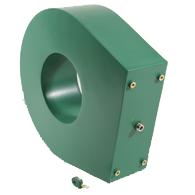
Range features
A high level overview of what this range offers
- 62 listed variants – Supports selection across a broad range of electrical and mechanical requirements.
- 0.0005 to 10 V/A sensitivity range – Allows the output level to be matched to the expected current and measuring instrument.
- Peak-current ratings up to 1,000,000 A – Provides options for low-current signals and high-energy pulse measurements.
- Four construction categories – Offers standard-package, clamp-on, double-shielded and thin configurations.
- Initial pulse accuracy of ±1% or better – Supports amplitude measurement under the specified high-impedance load conditions.
- Defined droop, rise-time and I·t ratings – Helps assess pulse flatness, edge reproduction and magnetic saturation limits.
- Defined RMS, bandwidth and I/f ratings – Supports model selection for continuous sinusoidal current.
- 50 Ω coaxial connection – Provides compatibility with common laboratory measuring instruments and cables.
- Double-shielded options – Can help control electric-field coupling in suitable high-voltage installations.
- Clamp-on construction options – Allow placement around an existing conductor without passing it through a closed aperture.
Downloads
for Custom current monitors
What’s in this range?
All the variants in the range and a comparison of what they offer
Range specifications
| Specification | Range or value |
|---|---|
Product scope | 62 listed custom current monitor variants |
Measurement principle | Current-transformer monitoring |
Measured waveforms | Pulse, transient and continuous AC signals |
Steady-state DC measurement | Not supported |
Construction categories | Standard package, clamp-on, double-shielded and thin |
Initial pulse-response accuracy | ±1% or better unless otherwise stated |
Accuracy load condition | High-impedance input, typically 1 MΩ in parallel with 20 pF |
Output sensitivity | 0.0005 to 10 V/A |
Hole or aperture entries | 0.22 to 15 in, plus coaxial and 12 × 2 in formats |
Peak current | 10 to 1,000,000 A |
Droop | 0.02 to 35,000 %/ms; model-dependent |
Usable rise time | 1.5 to 2,000 ns |
Maximum I·t | 0.00005 to 480 A·s; model-dependent |
Maximum RMS current | 1 to 3,500 A; model-dependent |
Low-frequency −3 dB point | 0.03 to 100,000 Hz |
High-frequency −3 dB point | 0.2 to 250 MHz |
I/f limit | 0.00007 to 3,500 peak A/Hz; model-dependent |
Output connector | BNC unless otherwise noted; Type N where marked |
Recommended cable | 50 Ω coaxial cable |
Effect of a 50 Ω termination | Reduces the stated voltage sensitivity by one half |
Housing | Conductive and not electrically insulated |
Standard-package variant comparison
| Model | Output (V/A) | Hole ID (in) | Peak current (A) | Droop (%/ms) | Usable rise time (ns) | I·t max (A·s) | Max RMS current (A) | Low −3 dB (Hz) | High −3 dB (MHz) | I/f (peak A/Hz) |
|---|---|---|---|---|---|---|---|---|---|---|
5753 | 10 | 2.0 | 50 | 700 | 150 | 0.0005 | 4 | 1,000 | 3 | 0.004 |
5834 | 10 | 2.0 | 50 | 300 | 350 | 0.001 | 4 | 500 | 1 | 0.006 |
8600 | 10 | 2.0 | 10 | 35,000 | 3 | 0.00005 | 1 | 45,000 | 125 | 0.00007 |
2854 | 1 | 5.0 | 500 | 40 | 15 | 0.04 | 5 | 30 | 20 | 3.5 |
7737 | 1 | 10.75 | 500 | 500 | 40 | 0.006 | 35 | 750 | 9 | 0.003 |
8181 | 1 | 1.0 | 500 | 80 | 15 | 0.002 | 5 | 125 | 20 | 0.014 |
8122 | 1 | 2.0 | 500 | 4 | 400 | 0.1 | 40 | 6 | 1 | 0.6 |
6027 | 1 | Coaxial | 100 | 200 | 2 | 0.0004 | 2.5 | 300 | 200 | 0.0025 |
8440 | 1 | 3.5 | 500 | 3 | 350 | 0.25 | 75 | 4 | 1 | 1.5 |
804 | 0.1 | 2.0 | 5,000 | 50 | 20 | 0.5 | 75 | 30 | 20 | 3.5 |
804R | 0.1 | 2.0 | 5,000 | 12 | 20 | 0.6 | 75 | 20 | 20 | 3.5 |
8611 | 0.1 | 4.0 | 5,000 | 1.5 | 40 | 0.5 | 140 | 2 | 10 | 3 |
3363 | 0.1 | 5.0 | 5,000 | 90 | 40 | 1 | 150 | 120 | 10 | 7.5 |
3382 | 0.1 | 15.0 | 1,000 | 50 | 80 | 1.5 | 250 | 100 | 4 | 10 |
4285 | 0.1 | 10.75 | 5,000 | 1.5 | 50 | 0.4 | 300 | 2 | 7 | 5.7 |
5011 | 0.1 | 0.25 | 400 | 20 | 5 | 0.004 | 10 | 30 | 70 | 0.025 |
5673 | 0.1 | 2.0 | 5,000 | 100 | 9 | 0.15 | 100 | 150 | 40 | 1.1 |
8365 | 0.1 | 0.25 | 400 | 7 | 20 | 0.004 | 10 | 10 | 20 | 0.025 |
8606 | 0.05 | 10.75 | 10,000 | 0.5 | 75 | 3 | 600 | 1 | 5 | 21.2 |
2811A | 0.02 | 0.5 | 1,000 | 1 | 500 | 6 | 150 | 1.5 | 0.7 | 40 |
8535 | 0.01 | 1.0 | 25,000 | 0.3 | 25 | 0.6 | 120 | 0.5 | 15 | 4 |
4191 | 0.01 | 4.0 | 50,000 | 4 | 60 | 5 | 400 | 6 | 7 | 35 |
4994 | 0.01 | 2.0 | 50,000 | 3 | 100 | 4.5 | 200 | 5 | 4 | 25 |
5803 | 0.01 | 10.75 | 50,000 | 4 | 200 | 12 | 1,000 | 7 | 2 | 80 |
5624 | 0.01 | 2.0 | 20,000 | 9 | 25 | 2 | 150 | 12 | 20 | 12 |
7427A | 0.01 | 2.0 | 4,000 | 2 | 5 | 0.2 | 100 | 5 | 70 | 1.2 |
5008 | 0.01 | 0.5 | 50,000 | 6 | 150 | 2 | 150 | 10 | 3 | 12 |
8573 | 0.01 | 3.5 | 50,000 | 0.02 | 200 | 30 | 750 | 0.03 | 2 | 225 |
6247A | 0.005 | 4.0 | 100,000 | 2 | 350 | 20 | 1,500 | 3 | 1 | 120 |
4427 | 0.001 | 3.5 | 500,000 | 0.1 | 300 | 480 | 2,800 | 1 | 1.2 | 3,060 |
5623 | 0.001 | 2.0 | 200,000 | 1 | 200 | 15 | 400 | 1.5 | 2 | 90 |
3880 | 0.001 | 12 × 2 | 100,000 | 0.3 | 500 | 150 | 1,200 | 0.5 | 0.7 | 1,000 |
2445 | 0.001 | 14.5 | 500,000 | 1.5 | 300 | 40 | 3,000 | 3 | 2 | 250 |
4906 | 0.001 | 10.75 | 500,000 | 1 | 400 | 50 | 2,000 | 2 | 1.5 | 300 |
7561 | 0.0005 | 4.75 | 1,000,000 | 0.2 | 2,000 | 750 | 3,500 | 0.15 | 0.2 | 3,500 |
Clamp-on variant comparison
| Model | Output (V/A) | Hole ID (in) | Peak current (A) | Droop (%/ms) | Usable rise time (ns) | I·t max (A·s) | Max RMS current (A) | Low −3 dB (Hz) | High −3 dB (MHz) | I/f (peak A/Hz) |
|---|---|---|---|---|---|---|---|---|---|---|
8240 | 2 | 2.0 | 500 | n/a | 12 | n/a | n/a | 100,000 | 30 | n/a |
8546 | 1 | 2.0 | 500 | 10 | 600 | 0.15 | 50 | 15 | 0.5 | 1.1 |
8375 | 1 | 2.0 | 500 | 7,000 | 4 | 0.001 | 10 | 11,000 | 100 | 0.007 |
8536 | 1 | 9.0 | 500 | 750 | 75 | 0.007 | 25 | 1,250 | 5 | 0.04 |
8579 | 0.1 | 10.75 | 5,000 | 250 | 50 | 0.7 | 120 | 400 | 7 | 4.4 |
6996 | 0.1 | 2.0 | 5,000 | 1,040 | 25 | 0.5 | 100 | 2,000 | 20 | 3 |
8330 | 0.01 | 2.0 | 1,000 | 100 | 7 | 0.3 | 100 | 200 | 50 | 2.1 |
7325 | 0.01 | 3.5 | 50,000 | 3 | 200 | 400 | 100 | 5 | 2 | 140 |
5769 | 0.05 | 3.5 | 10,000 | 8 | 100 | 4 | 250 | 12 | 3.5 | 25 |
8688 | 0.005 | 3.5 | 100,000 | 1.5 | 25 | 50 | 320 | 1.5 | 2.5 | 320 |
8591 | 0.001 | 6.0 | 500,000 | 0.3 | 400 | 15 | 1,000 | 0.4 | 1 | 105 |
Double-shielded variant comparison
| Model | Output (V/A) | Hole ID (in) | Peak current (A) | Droop (%/ms) | Usable rise time (ns) | I·t max (A·s) | Max RMS current (A) | Low −3 dB (Hz) | High −3 dB (MHz) | I/f (peak A/Hz) |
|---|---|---|---|---|---|---|---|---|---|---|
7266 | 1 | 0.5 | 500 | 0.09 | 10 | 0.002 | 5 | 140 | 35 | 0.006 |
7305 | 1 | 1.75 | 500 | 0.08 | 20 | 0.005 | 7.5 | 125 | 20 | 0.017 |
3464 | 0.1 | 1.75 | 5,000 | 0.8 | 20 | 0.5 | 100 | 1 | 20 | 1.7 |
4936 | 0.1 | 0.5 | 5,000 | 0.9 | 20 | 0.2 | 50 | 1 | 20 | 0.6 |
5007 | 0.01 | 1.75 | 20,000 | 0.3 | 20 | 1 | 150 | 0.5 | 20 | 3.5 |
5405 | 0.01 | 0.5 | 50,000 | 6 | 150 | 2 | 150 | 10 | 3 | 12 |
8574 | 0.025 | 1.75 | 20,000 | 100 | 100 | 0.5 | 100 | 160 | 4 | 3 |
Thin-model variant comparison
| Model | Output (V/A) | Hole ID (in) | Peak current (A) | Droop (%/ms) | Usable rise time (ns) | I·t max (A·s) | Max RMS current (A) | Low −3 dB (Hz) | High −3 dB (MHz) | I/f (peak A/Hz) |
|---|---|---|---|---|---|---|---|---|---|---|
7713-03 | 1 | 0.22 | 100 | 600 | 1.5 | 0.0002 | 2 | 1,000 | 250 | 0.0014 |
8105-03 | 0.1 | 0.22 | 300 | 50 | 10 | 0.002 | 6 | 50 | 40 | 0.013 |
5974 | 0.1 | 0.5 | 5,000 | 1 | 20 | 0.15 | 50 | 2 | 20 | 0.6 |
8500 | 0.1 | 2.0 | 5,000 | 4 | 20 | 0.1 | 75 | 10 | 20 | 0.6 |
8445 | 0.1 | 2.0 | 5,000 | 4 | 20 | 0.1 | 75 | 10 | 20 | 0.6 |
8568 | 0.01 | 0.5 | 25,000 | 0.4 | 25 | 0.4 | 100 | 0.8 | 15 | 2.5 |
8532 | 0.01 | 1.0 | 10,000 | 0.5 | 25 | 0.5 | 100 | 0.7 | 15 | 3 |
7765 | 0.01 | 2.0 | 20,000 | 1 | 25 | 0.25 | 150 | 1 | 20 | 1 |
6535-03 | 0.005 | 0.22 | 5,000 | 1.5 | 20 | 0.04 | 30 | 2.5 | 20 | 0.25 |
The listed output values apply with a high-impedance load. A 50 Ω termination reduces the voltage output by one half. Droop describes the initial decay of the output during a flat-top current pulse, while usable rise time is the 10–90% transition that limits initial overshoot to less than 10%.
FAQs
for Custom current monitors
Start by defining the expected peak current, pulse duration, repetition rate and 10–90% rise time. Both the peak-current rating and the I·t limit must remain above the application values, because a monitor can satisfy the peak rating yet still saturate when the pulse lasts too long. Choose a usable rise-time specification shorter than the signal rise time, then estimate flat-top deviation by multiplying droop in %/ms by the pulse duration in milliseconds. Check that the selected sensitivity produces a practical voltage without overdriving the output or measuring instrument. Finally, confirm that the conductor, insulation and required clearances fit through the stated aperture.
No, steady-state DC is not reproduced because the output depends on changing magnetic flux in the current-transformer core. A DC component or repetitive unipolar pulse train can progressively bias the core, increasing droop and the low-frequency cut-off while reducing the available I·t capacity. Biasing can sometimes be introduced through additional turns in the aperture or through a coaxial T-adaptor to reset the operating flux point. Individual DC-bias limits are not included in the custom-range data, so they require application-specific confirmation. In practice, selection should account for average current and pulse repetition as well as peak amplitude and pulse width.
The stated sensitivity applies with a high-impedance input, typically around 1 MΩ in parallel with 20 pF. The monitor generally behaves as a voltage source with approximately 50 Ω series impedance, so a 50 Ω instrument termination forms a two-to-one voltage divider. A model rated at 1 V/A will therefore produce approximately 0.5 V/A at the terminated input. Matched termination can improve pulse-edge fidelity when the connecting cable is electrically long compared with the fastest signal component. The reduced sensitivity must be included in current calculations, calibration settings and instrument scaling.
Standard-package models suit installations where the conductor can be passed through a closed aperture during assembly. Clamp-on models separate into two sections, allowing placement around an existing conductor, although their plug-and-socket contacts must be handled carefully when opening and closing the unit. Thin models are intended for locations where axial installation space is restricted, while double-shielded variants can help reduce electric-field coupling. Large-aperture constructions may be suitable for high-voltage conductors when the required insulation and clearances are provided. Selection should consider aperture dimensions, conductor routing, access, shielding, earthing and mechanical support together.
Droop describes the initial downward slope of the output during a constant-current portion of the pulse. As a practical approximation, multiply the specified droop in %/ms by the pulse duration in milliseconds to estimate the output change across the flat top. A model rated at 0.02%/ms would produce approximately 0.02% deviation during a 1 ms pulse, while a high-droop model is intended for much shorter events. Lower droop normally corresponds to a lower low-frequency cut-off, but it can involve trade-offs in rise time, physical size or sensitivity. Model selection should therefore be based on the actual pulse width rather than peak current alone.
Usable rise time is the 10–90% current transition that produces no more than 10% initial overshoot or ringing in the output. The selected monitor should have a stated usable rise time shorter than the rise time of the signal being measured. Across the range, listed values extend from 1.5 to 2,000 ns, while high-frequency −3 dB points extend from 0.2 to 250 MHz. The −3 dB bandwidth alone does not fully describe pulse behaviour, so the time-domain rise specification should also be checked. Faster models may trade low-frequency response, I·t capacity or RMS-current capability for improved edge reproduction.
For sinusoidal signals, check the low and high −3 dB points, maximum RMS current and I/f limit. The signal frequency must remain within the stated bandwidth, while RMS current must remain below the thermal rating. Divide the expected peak current by the lowest operating frequency and compare the result with the model’s I/f value; for example, an I/f rating of 3 A/Hz permits 300 A peak at 100 Hz, subject to the RMS limit. The listed range covers low-frequency points from 0.03 to 100,000 Hz and upper points from 0.2 to 250 MHz. Always evaluate the lowest operating frequency because the I/f demand increases as frequency falls.
The housing is conductive and its painted finish does not provide electrical insulation. The monitor must never be mounted, removed or opened around an energised conductor, and the conductor insulation must withstand the full voltage difference between the circuit and the housing. In single-shielded constructions, the shield is normally connected to the output connector and coaxial braid, which can establish a path to the instrument earth. Double-shielded models provide separate outer-shield earthing options through their mounting arrangement. The complete installation should therefore be checked for insulation, clearance, earthing, cable routing and accessible conductive parts before energisation.