Wideband current monitors
- Technology
- Photonics accessories
- Partner
- Pearson Electronics
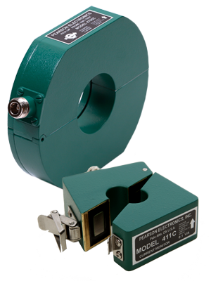
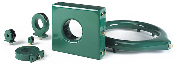
This 30-model product range uses current-transformer coupling around a conductor passed through the monitor aperture, producing a proportional voltage without inserting a conventional current-viewing resistor into the primary circuit. The monitors measure pulse currents, transients and continuous AC signals, but do not reproduce steady-state DC. Applications include low-level beam current measurement, high-energy surge testing, power-system harmonics, EMI investigation, plasma work, capacitive discharge, lightning studies and pulsed equipment. Sensitivities from 1 V/A to 0.001 V/A allow the output to be matched to the expected current and measuring-instrument input range.
Aperture diameters from 0.25 to 10.75 inches accommodate different conductors, busbars, insulation requirements and installation geometries. Model-dependent peak-current ratings extend from 100 A to 500 kA, with usable rise times from 1.5 ns to 2 µs. Sealed construction and selected double-shielded variants support high-voltage, vacuum, insulating-oil and electrically noisy environments, subject to correct insulation and grounding.
Range features
A high level overview of what this range offers
- Thirty model variants: Supports selection around pulse, frequency, sensitivity and installation requirements.
- Sensitivity from 1 to 0.001 V/A: Matches different current levels and measuring-instrument input ranges.
- Peak ratings from 100 A to 500 kA: Covers low-current pulse analysis through high-energy transient measurement.
- Usable rise times from 1.5 ns to 2 µs: Provides options for fast pulse edges and lower-bandwidth, high-current events.
- Apertures from 0.25 to 10.75 inches: Accommodates different conductors, busbars and insulation arrangements.
- Through-aperture magnetic coupling: Avoids direct electrical connection to the measured conductor and keeps insertion resistance low.
- Selected double-shielded models: Helps reduce electric-field pickup in high-voltage or electrically noisy installations.
- Sealed construction: Permits installation in insulating oil or under vacuum.
- Multiple connector formats: Supports BNC, SMA, UHF and Type N measurement connections, depending on the model.
- Broad instrument compatibility: Connects to oscilloscopes, spectrum analysers, network analysers, power analysers, voltmeters and digitising systems.
Downloads
for Wideband current monitors
What’s in this range?
All the variants in the range and a comparison of what they offer
Range Specifications
| Specification | Range details |
|---|---|
Sensitivity | 0.001 to 1 V/A |
Aperture diameter | 0.25 to 10.75 inches |
Maximum peak current | 100 to 500,000 A, model-dependent |
Maximum RMS current | 2.5 to 2,500 A, model-dependent |
Usable rise time | 1.5 ns to 2 µs, model-dependent |
Droop | 0.05 to 300%/ms, model-dependent |
Maximum current-time product | 0.0004 to 1,200 A·s |
Low-frequency 3 dB points | 0.07 to 400 Hz across the range |
High-frequency 3 dB points | 0.2 to 250 MHz across the range |
I/f limit | 0.0025 to 7,500 peak A/Hz |
Initial pulse-amplitude tolerance | Model-specific: +1/-0% or ±1% with a high-impedance load |
Output source resistance | Usually 50 Ω; Model 2093 is specified at 1 Ω |
External 50 Ω termination | Halves nominal sensitivity on models with a 50 Ω source resistance |
Shielding | Single or double, depending on model |
Construction | Sealed; suitable for insulating oil or vacuum |
Model Comparison
| Specification | 2877 | 4100 | 2100 | 6585 | 6656 | 3100¹ | 150 | 6595 | 325¹ | 2878 | 410 | 411 | 3972 | 110 | 110A² | 6600 | 310¹ | 1010¹ | 1025 | 3025¹ | 2879 | 5046 | 101 | 4997 | 301X¹ | 1080¹² | 1330¹ | 4418 | 1423¹ | 2093¹ |
|---|---|---|---|---|---|---|---|---|---|---|---|---|---|---|---|---|---|---|---|---|---|---|---|---|---|---|---|---|---|---|
Shape | F | E | D | K | J | C | D | K | C | F | E | E | I | D | D | K | C | A | D | C | F | E | D | D | C | C | C | D | C | B |
Output (V/A) | 1.0 | 1.0 | 1.0 | 1.0 | 1.0 | 1.0 | 0.5 | 0.5 | 0.25 | 0.1 | 0.1 | 0.1 | 0.1 | 0.1 | 0.1 | 0.1 | 0.1 | 0.1 | 0.025 | 0.025 | 0.01 | 0.01 | 0.01 | 0.01 | 0.01 | 0.005 | 0.005 | 0.001 | 0.001 | 0.001 |
Aperture (inches) | 0.25 | 0.5 | 2.0 | 2.0 | 3.5 | 3.5 | 2.0 | 2.0 | 3.5 | 0.25 | 0.5 | 0.5 | 1.0 | 2.0 | 2.0 | 2.0 | 3.5 | 10.75 | 2.0 | 3.5 | 0.25 | 0.5 | 2.0 | 2.0 | 3.5 | 3.5 | 3.5 | 2.0 | 3.5 | 4.75 |
Maximum peak current (A) | 100 | 500 | 500 | 500 | 500 | 500 | 1,000 | 1,000 | 2,000 | 400 | 5,000 | 5,000 | 5,000 | 5,000 | 10,000 | 2,000 | 5,000 | 5,000 | 20,000 | 20,000 | 2,000 | 25,000 | 50,000 | 20,000 | 50,000 | 200,000 | 100,000 | 200,000 | 500,000 | 500,000 |
Droop (%/ms) | 200 | 90 | 80 | 300 | 140 | 40 | 20 | 100 | 100 | 20 | 60 | 0.9 | 1 | 0.8 | 0.8 | 15 | 20 | 250 | 100 | 4 | 2 | 0.3 | 0.1 | 0.3 | 3 | 2.0 | 1.0 | 0.05 | 0.7 | 0.09 |
Usable rise time (ns) | 2 | 10 | 20 | 1.5 | 3.5 | 50 | 20 | 2.5 | 30 | 5 | 20 | 20 | 20 | 20 | 20 | 5 | 40 | 50 | 100 | 100 | 20 | 20 | 100 | 25 | 200 | 250 | 250 | 200 | 500 | 2,000 |
Maximum I·t (A·s) | 0.0004³ | 0.002³ | 0.005³ | 0.002³ | 0.01³ | 0.03³ | 0.02³ | 0.008³ | 0.09 | 0.004³ | 0.25 | 0.2³ | 0.2 | 0.5³ | 0.5³ | 0.04³ | 0.6 | 0.7³ | 0.5 | 3.0 | 0.04³ | 0.5³ | 2.5³ | 1.0³ | 22 | 25 | 65 | 6.0³ | 75 | 1,200 |
Maximum RMS current (A) | 2.5 | 5 | 7.5 | 10 | 10 | 12 | 15 | 20 | 60 | 10 | 50 | 50 | 50 | 65 | 65 | 40 | 140 | 120 | 100 | 325 | 25 | 100 | 200 | 150 | 400 | 750 | 1,400 | 400 | 2,500 | 2,500 |
Low 3 dB point (Hz) | 300 | 140 | 125 | 400 | 200 | 40 | 40 | 100 | 160 | 30 | 120 | 1 | 1 | 1 | 1 | 25 | 40 | 400 | 160 | 7 | 3 | 0.5 | 0.25 | 0.5 | 5 | 3.0 | 0.9 | 0.07 | 1.0 | 0.15 |
High 3 dB point (MHz) | 200 | 35 | 20 | 250 | 120 | 7 | 20 | 200 | 10 | 70 | 20 | 20 | 20 | 20 | 20 | 120 | 10 | 7 | 4 | 4 | 20 | 20 | 4 | 15 | 2 | 1.5 | 1.5 | 2 | 1.2 | 0.2 |
I/f limit (peak A/Hz) | 0.0025 | 0.006 | 0.017 | 0.008 | 0.04 | 0.1 | 0.07 | 0.03 | 0.6 | 0.025 | 1.7 | 0.6 | 0.6 | 1.5 | 1.5 | 0.12 | 3.6 | 4.4 | 3.0 | 20.0 | 0.25 | 3.0 | 12.0 | 3.5 | 140.0 | 150 | 400 | 40 | 450 | 7,500 |
¹ Double-shielded model. ² Type N output connector. ³ A small DC bias current through the secondary may be required to obtain the stated maximum current-time rating.
Shape letters identify the available case formats. Detailed mechanical dimensions should be taken from the dimensional drawing for the selected model rather than inferred from the shape code.
FAQs
for Wideband current monitors
Start with peak current, current-time product, rise time and droop; sensitivity should be considered after those limits are satisfied. For a rectangular pulse, multiply peak current by pulse duration and choose a model whose I·t rating exceeds the result while also remaining below its peak rating; across the range, these limits run from 0.0004 to 1,200 A·s and 100 A to 500 kA. Estimate flat-top error by multiplying pulse duration by droop rate using consistent time units. The pulse’s 10–90% rise time should be longer than the monitor’s usable rise-time rating, which spans 1.5 ns to 2 µs by model. Once these conditions are met, select the sensitivity and aperture that provide a practical output voltage and fit the insulated conductor.
For continuous sine-wave current, selection is governed by RMS current, frequency band and I/f rather than peak rating alone. Divide peak current by the lowest operating frequency and keep the result below the selected model’s I/f limit, which ranges from 0.0025 to 7,500 peak A/Hz across the range. The expected RMS current must also remain below the model rating of 2.5 to 2,500 A. Operation should remain between that model’s low and high 3 dB points; the collective range extends from 0.07 Hz to 250 MHz, but no single model covers the entire span. Finally, confirm that the selected sensitivity produces enough voltage for the measuring instrument without overloading its input.
Use a high-impedance input when the nominal V/A sensitivity must be retained. Most models behave approximately as voltage sources with 50 Ω series resistance, so adding a 50 Ω termination reduces the measured voltage and effective sensitivity to one half; Model 2093 is an exception with a 1 Ω output resistance. A matched termination can nevertheless improve pulse-edge fidelity when the coaxial cable is electrically long relative to the fastest signal, typically beyond about one tenth of its wavelength. The current calculation must therefore include the termination ratio as well as the stated sensitivity. Cable type, connector family and oscilloscope input mode should be fixed before the scaling is entered into the acquisition system.
The monitors do not reproduce steady-state DC because their output depends on changing magnetic flux. A repetitive unipolar pulse train contains an average DC component, so the displayed waveform can show a negative baseline even when the primary current never becomes negative. That average component, together with the pulse I·t, can drive the core towards saturation, increasing droop and the low-frequency cut-off before the waveform collapses. Core-reset bias can be used on suitable models to counter the average component or recover more usable flux swing. The design should therefore be checked against duty cycle, average current and I·t, not only the peak value of each pulse.
High-voltage use requires the primary conductor to be insulated for the full potential difference because the monitor case is conductive and its paint is not an electrical insulation system. Larger apertures, including 3.5- and 10.75-inch options, provide space for insulation and help control electric-field gradients when the conductor is centred. Selected models are double shielded, allowing the outer case to be grounded through mounting hardware while the inner shield and connector can be referenced at the instrument or another suitable point. The sealed construction permits installation in transformer oil or under vacuum, but creepage distance, cleanliness and barrier materials remain part of the system design. Installation or removal should never be attempted on a live conductor.
Usable rise time is the fastest 10–90% current transition that the monitor can reproduce while keeping overshoot and ringing within 10% of the step amplitude. The selected monitor should therefore have a specified rise time shorter than the pulse being measured; using a slower monitor can round the edge or introduce ringing that obscures switching behaviour. Available ratings range from 1.5 ns for fast variants to 2 µs for high-current, lower-bandwidth models. The oscilloscope, cable, adaptors and any termination must also have adequate bandwidth, otherwise the system rise time will be slower than the monitor alone. For timing-critical measurements, evaluate the complete signal chain rather than selecting from the high-frequency 3 dB point only.
The primary-circuit disturbance is generally small, but it is not exactly zero. Standard models introduce less than 20 mΩ of equivalent series resistance, and the magnetic coupling can slightly reduce loop inductance because the secondary ampere-turns oppose part of the primary flux. In fast, low-inductance circuits, that change may need to be included in the measurement-fixture assessment. Capacitively coupled common-mode noise can also travel on the coaxial cable shield and appear at the instrument input. Correct grounding, a double-shielded model where appropriate, and one or more ferrite cores around turns of the coaxial cable can reduce this error.
Biasing is relevant when a model is marked as requiring it for the full current-time rating, or when repetitive unidirectional current creates an average component that moves the core towards saturation. A suitable bias resets the magnetic operating point, allowing more flux swing and helping the monitor maintain its specified droop and I·t behaviour. It may be applied through an additional primary conductor or injected into the secondary through a T adaptor, provided the bias source does not load the signal output. For a 50 Ω output, a 5 kΩ bias-source resistance corresponds to about a 1% sensitivity shift, which should be included in the uncertainty budget. Biasing does not increase the I/f capability for a pure AC signal because its positive and negative flux excursions are already balanced.