Clamp-on current monitors
- Technology
- Photonics accessories
- Partner
- Pearson Electronics
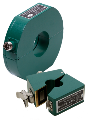
These clamp-on current monitors use separable magnetic-core assemblies that fit around an existing conductor without requiring it to be disconnected. They convert changing current into a proportional voltage for measurement with an oscilloscope, digitiser, voltmeter, spectrum analyser or network analyser. The 21-model range offers sensitivities from 1.0 to 0.001 V/A and conductor apertures from 0.5 to 6.0 inches. Applications include pulse-current testing, EMI measurement, RF and video currents, power-system transients, lightning testing, welding equipment, plasma research and charged-particle beam instrumentation.
Model selection depends on peak current, current-time product, usable rise time, droop, RMS current, frequency range and I/f capability. Because these are transformer-based devices, they reproduce changing current but cannot measure steady-state DC. The conductive case is not electrically insulated, so the conductor must have adequate insulation and must be de-energised before the monitor is installed, opened or removed.
Range features
A high level overview of what this range offers
- Separable two-part construction: Allows the monitor to be fitted around an existing conductor.
- 21 model options: Supports selection for different current levels, waveform speeds and conductor sizes.
- 1.0 to 0.001 V/A sensitivity range: Matches the output level to the expected current and instrument input range.
- 0.5 to 6.0-inch apertures: Accommodates cables, conductors and larger current paths.
- 1 to 250 ns usable rise time: Provides model choices for fast pulse and transient measurements.
- 15 to 200,000 A peak-current ratings: Covers low-current probe applications through high-energy pulse testing.
- 4 to 500 A RMS-current ratings: Supports continuous AC and repetitive waveform measurement within model limits.
- Transformer coupling: Avoids inserting a conventional current-viewing shunt into the measured circuit.
- ±1% or better initial pulse response: Provides defined amplitude accuracy under the stated high-impedance loading conditions.
- 50 Ω output architecture: Connects to standard coaxial measurement equipment and termination systems.
- Model-specific I·t and I/f ratings: Identifies core-saturation limits for pulse and sinusoidal waveforms.
- BNC or Type N connection: Provides established interfaces for laboratory and compliance-test equipment.
Downloads
for Clamp-on current monitors
What’s in this range?
All the variants in the range and a comparison of what they offer
Specifications
| Parameter | Specification |
|---|---|
Number of models | 21 |
Measurement types | Pulses, transients and continuous AC signals |
Steady-state DC measurement | Not supported |
Initial pulse-response accuracy | ±1% or better unless otherwise stated, with approximately 1 MΩ in parallel with 20 pF |
Output sensitivity | 1.0, 0.5, 0.1, 0.01 or 0.001 V/A |
Output source resistance | 50 Ω where specified in the individual model data |
Output connector | BNC on most models; Type N where noted |
Recommended cable | 50 Ω coaxial cable |
Effect of 50 Ω termination | Reduces the output voltage to approximately half the high-impedance value |
Conductor aperture | 0.5 to 6.0 inches |
Maximum peak current | 15 to 200,000 A |
Maximum RMS current | 4 to 500 A |
Droop rate | 0.00025 to 4%/µs |
Usable rise time | 1 to 250 ns |
Maximum current-time product | 0.0006 to 8 A·s |
Low-frequency 3 dB point | 0.4 to 1,500 Hz |
High-frequency 3 dB point | 1.5 to 400 MHz |
I/f rating | 0.002 to 50 RMS A/Hz in the range comparison |
Maximum I²t | 0.02 to 2,000,000 A²s |
Operating temperature | 0 to 65°C where stated for the individual model |
Variant range comparison
| Model | Shape | Output V/A | Hole ID in | Peak current A | Droop %/µs | Rise time ns | I·t max A·s | RMS current A | Low 3 dB Hz | High 3 dB MHz | I/f RMS A/Hz | I²t max A²s |
|---|---|---|---|---|---|---|---|---|---|---|---|---|
8585C | N | 1.0 | 0.5 | 500 | 1.0 | 2 | 0.003 | 5 | 1,500 | 200 | 0.01 | 5 |
4100C | N | 1.0 | 0.5 | 500 | 1.0 | 15 | 0.0015 | 5 | 1,500 | 25 | 0.008 | 150 |
8590C | M | 1.0 | 1.0 | 500 | 0.7 | 2.5 | 0.002 | 5 | 1,000 | 150 | 0.01 | 25 |
7790 | M | 1.0 | 1.0 | 500 | 1.0 | 15 | 0.002 | 5 | 1,500 | 25 | 0.01 | 150 |
4688 | L | 1.0 | 2.0 | 500 | 0.4 | 12 | 0.005 | 15 | 600 | 30 | 0.03 | 150 |
8705C | — | 1.0 | 2.0 | 15 | 4.0 | 1 | 0.0006 | 4 | 1,500 | 400 | 0.002 | 0.02 |
7805 | K | 1.0 | 4.0 | 500 | 0.7 | 25 | 0.004 | 15 | 1,000 | 25 | 0.02 | 150 |
7760 | J | 1.0 | 6.0 | 500 | 0.5 | 50 | 0.005 | 20 | 750 | 7.0 | 0.03 | 350 |
5101 | L | 0.5 | 2.0 | 1,000 | 0.1 | 20 | 0.02 | 25 | 150 | 18 | 0.08 | 700 |
5949 | K | 0.5 | 4.0 | 1,000 | 0.1 | 30 | 0.02 | 30 | 150 | 12 | 0.08 | 700 |
411C | N | 0.1 | 0.5 | 5,000 | 0.015 | 20 | 0.15 | 50 | 25 | 20 | 0.7 | 18,000 |
7795 | M | 0.1 | 1.0 | 5,000 | 0.015 | 25 | 0.15 | 60 | 25 | 15 | 0.8 | 18,000 |
3525 | L | 0.1 | 2.0 | 5,000 | 0.004 | 25 | 0.5 | 100 | 6.0 | 15 | 2.5 | 18,000 |
7810 | K | 0.1 | 4.0 | 5,000 | 0.007 | 50 | 0.4 | 150 | 10 | 7.0 | 2.0 | 18,000 |
7655 | J | 0.1 | 6.0 | 5,000 | 0.007 | 100 | 0.4 | 175 | 10 | 4.0 | 2.0 | 35,000 |
5008C | N | 0.01 | 0.5 | 50,000 | 0.005 | 150 | 1.0 | 150 | 7.5 | 3.0 | 4.2 | 250,000 |
7800 | M | 0.01 | 1.0 | 50,000 | 0.003 | 175 | 0.8 | 125 | 5.0 | 2.0 | 4.0 | 140,000 |
4160 | L | 0.01 | 2.0 | 50,000 | 0.001 | 200 | 2.5 | 300 | 1.5 | 2.0 | 15.0 | 1,000,000 |
7815 | K | 0.01 | 4.0 | 50,000 | 0.001 | 200 | 3.0 | 400 | 1.5 | 2.0 | 15.0 | 2,000,000 |
7450 | J | 0.01 | 6.0 | 50,000 | 0.001 | 250 | 3.0 | 400 | 1.5 | 1.5 | 12 | 2,000,000 |
5664 | L | 0.001 | 2.0 | 200,000 | 0.00025 | 250 | 8.0 | 500 | 0.4 | 1.5 | 50 | 1,000,000 |
Document-control note: Some comparison values differ from the corresponding detailed model records. Model 5949 is also documented with a 2,000 A peak rating, a 175 Hz low-frequency point and a Type N connector. Model 3525 is also documented with a 5 Hz low-frequency point, while Model 5008C is also documented with 10%/ms droop and a 15 Hz low-frequency point. Model 5664 is also listed with an I/f value of 35 RMS A/Hz. Model 8705C is characterised as an EMI probe with a nominal terminated transfer impedance of −6 dBΩ and a stated operating range of 10 kHz to 400 MHz. Confirm the applicable model datasheet values before final specification or test-procedure approval.
Safety: The painted conductive case does not provide electrical insulation. Do not install, open or remove a monitor while the conductor is energised.
FAQs
for Clamp-on current monitors
Start with the expected peak current, pulse duration and 10–90% rise time. Multiply the current by the pulse duration and select a model whose peak-current and I·t ratings both exceed the resulting values; for example, a 2,000 A pulse lasting 100 µs has an I·t of 0.2 A·s. The monitor’s usable rise time should be shorter than the measured transition to control overshoot and ringing. Next, multiply the specified droop rate by the pulse duration in microseconds to estimate flat-top deviation. Sensitivity and aperture size should only be considered after these electrical limits have been satisfied.
Check the maximum RMS current, the low and high 3 dB points, and the I/f rating. For example, a 100 A peak sine wave at 50 Hz produces an I/f value of 2 A/Hz and an RMS current of approximately 70.7 A. The selected model must accommodate both figures while keeping 50 Hz within its stated frequency band. Operation close to either 3 dB point introduces additional amplitude and phase error, so margin from the frequency limits is desirable. If the signal contains harmonics, repeat the frequency and heating assessment for the highest relevant harmonic content.
Use a high-impedance instrument input when the full stated V/A sensitivity is required. A 50 Ω termination is useful for pulses with rise times below approximately 100 ns, RF measurements above a few megahertz or installations using electrically long coaxial cables, because it reduces reflections and cable fill-time effects. With a 50 Ω source and 50 Ω load, the measured voltage is approximately half the high-impedance value. Cable attenuation and termination tolerance must also be included in the current conversion. The acquisition system should therefore be configured for either terminated or unterminated sensitivity before measurements begin.
They cannot measure steady-state DC because the operating principle is based on changing magnetic flux. A repetitive unipolar pulse train contains an average DC component even though each individual pulse is time-varying. This average component can move the magnetic core towards saturation, increasing droop and the low-frequency cut-off while reducing the available I·t capability. Biasing can support some applications by resetting or offsetting the core flux, but the required arrangement must be assessed for the particular monitor and waveform. In practice, calculate the average current and pulse area rather than evaluating peak current alone.
Choose an aperture that clears the conductor and its complete insulation system without forcing the monitor against the live insulation surface. The available hole diameters range from 0.5 to 6.0 inches, but aperture size does not itself establish a safe operating voltage. The monitor case is conductive and its painted finish must not be treated as electrical insulation. Never install, open or remove the monitor while the conductor is energised. Creepage distance, clearance, conductor centring, insulation barriers, earthing and the surrounding environment must all be addressed by the equipment or test-system design.
Select a monitor whose usable rise time is shorter than the rise time of the current transition being measured. Across the range, usable rise-time ratings extend from 1 to 250 ns and represent the fastest 10–90% transition that keeps overshoot and ringing within approximately 10%. For frequencies at least one decade away from both cut-off points, phase shift is usually below 6 degrees and amplitude error below 1%. Performance becomes less predictable as the signal approaches the low or high 3 dB boundary. Timing-sensitive work should therefore consider rise time, bandwidth, phase response, cable length and oscilloscope bandwidth together.
The I²t rating represents the transient-energy limit associated with heating in the monitor’s internal secondary circuit. For a constant-amplitude pulse, it can be estimated as current squared multiplied by duration; a 500 A pulse lasting 1 ms therefore produces 250 A²s. The selected monitor’s I²t limit must exceed the calculated value with suitable allowance for waveform uncertainty and repetition. Core saturation may limit secondary energy during some unidirectional events, but it should not be used as the primary protection method. Bidirectional and oscillatory transients require particular attention because their energy is not limited in the same way by one-direction core saturation.
With a high-impedance input, the output voltage is the measured primary current multiplied by the monitor sensitivity. A 1 V/A model produces 10 V for a 10 A current, while a 0.01 V/A model produces 0.1 V for the same current. Adding a 50 Ω termination reduces these outputs to approximately 5 V and 0.05 V respectively. Passing the conductor through the aperture twice doubles the effective sensitivity, but it also halves the available I·t and I/f ratings. Peak-current, RMS-current, aperture and instrument-input limits must therefore be rechecked whenever multiple primary passes are used.